범주형 독립변수
Contents
3.13. 범주형 독립변수#
이 절에서는 선형회귀분석에 있어서 범주형 독립변수(categorical independent variable)의 사용법을 공부한다.
예제로는 팁 데이터와 보스턴 집값 데이터를 사용한다.
import seaborn as sns

tips = sns.load_dataset("tips").sample(frac=1, random_state=0).reset_index(drop=True)
tips.head()
| total_bill | tip | sex | smoker | day | time | size | |
|---|---|---|---|---|---|---|---|
| 0 | 17.59 | 2.64 | Male | No | Sat | Dinner | 3 |
| 1 | 18.29 | 3.76 | Male | Yes | Sat | Dinner | 4 |
| 2 | 19.49 | 3.51 | Male | No | Sun | Dinner | 2 |
| 3 | 7.25 | 1.00 | Female | No | Sat | Dinner | 1 |
| 4 | 16.27 | 2.50 | Female | Yes | Fri | Lunch | 2 |
import statsmodels.api as sm

boston = sm.datasets.get_rdataset("Boston", "MASS").data
boston.head()
| crim | zn | indus | chas | nox | rm | age | dis | rad | tax | ptratio | black | lstat | medv | |
|---|---|---|---|---|---|---|---|---|---|---|---|---|---|---|
| 0 | 0.00632 | 18.0 | 2.31 | 0 | 0.538 | 6.575 | 65.2 | 4.0900 | 1 | 296 | 15.3 | 396.90 | 4.98 | 24.0 |
| 1 | 0.02731 | 0.0 | 7.07 | 0 | 0.469 | 6.421 | 78.9 | 4.9671 | 2 | 242 | 17.8 | 396.90 | 9.14 | 21.6 |
| 2 | 0.02729 | 0.0 | 7.07 | 0 | 0.469 | 7.185 | 61.1 | 4.9671 | 2 | 242 | 17.8 | 392.83 | 4.03 | 34.7 |
| 3 | 0.03237 | 0.0 | 2.18 | 0 | 0.458 | 6.998 | 45.8 | 6.0622 | 3 | 222 | 18.7 | 394.63 | 2.94 | 33.4 |
| 4 | 0.06905 | 0.0 | 2.18 | 0 | 0.458 | 7.147 | 54.2 | 6.0622 | 3 | 222 | 18.7 | 396.90 | 5.33 | 36.2 |
3.13.1. 레벨이 2개인 범주형 독립변수#
범주형 독립변수가 가질 수 있는 값을 레벨(level)이라고 한다. 우선 가장 간단한 모형으로 레벨이 2개인 범주형 독립변수만을 가지는 선형회귀모형을 살펴보자. 예를 들어 팁 데이터에서 time 변수는 Lunch와 Dinner라는 두가지 레벨을 가지는 독립변수이고 sex 변수도 남성 Male과 Female이라는 두 가지 레벨을 가지는 독립변수다. 우선 time 변수로 팁 데이터를 예측하는 선형회귀모형을 만들어보자.
단 하나의 범주형 독립변수를 사용할 경우 두 가지 선형회귀모형을 만들어 볼 수 있다. 각각의 모형 문자열은 다음과 같다.
모형 1 :
tip ~ C(time) + 0모형 2 :
tip ~ C(time)
model1 = sm.OLS.from_formula("tip ~ C(time) + 0", tips)
model2 = sm.OLS.from_formula("tip ~ C(time)", tips)
이 두가지 모형이 각각 어떤 의미인지를 파악하기 위해 각각 범주형 변수의 값(레벨)이 어떤 숫자로 인코딩되는지를 살펴보자.
import pandas as pd

X0 = tips[["time"]]
X1 = pd.DataFrame(model1.exog, columns=model1.exog_names).head(10).astype(int)
X2 = pd.DataFrame(model2.exog, columns=model2.exog_names).head(10).astype(int)
pd.concat([X0, X1, X2], axis=1, keys=["raw", "model1", "model2"]).head(10).style.background_gradient(vmin=0, vmax=1)
| raw | model1 | model2 | |||
|---|---|---|---|---|---|
| time | C(time)[Lunch] | C(time)[Dinner] | Intercept | C(time)[T.Dinner] | |
| 0 | Dinner | 0.000000 | 1.000000 | 1.000000 | 1.000000 |
| 1 | Dinner | 0.000000 | 1.000000 | 1.000000 | 1.000000 |
| 2 | Dinner | 0.000000 | 1.000000 | 1.000000 | 1.000000 |
| 3 | Dinner | 0.000000 | 1.000000 | 1.000000 | 1.000000 |
| 4 | Lunch | 1.000000 | 0.000000 | 1.000000 | 0.000000 |
| 5 | Dinner | 0.000000 | 1.000000 | 1.000000 | 1.000000 |
| 6 | Dinner | 0.000000 | 1.000000 | 1.000000 | 1.000000 |
| 7 | Dinner | 0.000000 | 1.000000 | 1.000000 | 1.000000 |
| 8 | Dinner | 0.000000 | 1.000000 | 1.000000 | 1.000000 |
| 9 | Dinner | 0.000000 | 1.000000 | 1.000000 | 1.000000 |
모형1에서는 C(time)[Lunch] 와 C(time)[Dinner] 라는 두 개의 변수가 만들어지고 이 값은 각각 다음과 같이 인코딩되었다. 모형2에서는 Intercept 와 C(time)[T.Dinner] 라는 두 개의 변수가 만들어지고 이 값은 각각 다음과 같이 인코딩되었다.
이렇게 범주형 독립변수를 선형회귀분석에 사용하게 되면 레벨의 개수와 같은 개수의 변수가 만들어지는데 이를 더미변수(dummy variable)라고 한다. 더미변수의 값은 0 또는 1 값만을 가질 수 있다. 더미변수의 값을 정하는 규칙을 더미변수 인코딩(encoding) 규칙이라고 한다.
모형1에서 더미변수의 값은 다음과 같이 정해진다.
Lunch -> C(time)[Lunch] = 1, C(time)[T.Dinner] = 0
Dinner -> C(time)[Lunch] = 0, C(time)[T.Dinner] = 1
즉 C(time)[Lunch] 변수를 \(d_L\), 그 가중치를 \(w_L\), C(time)[T.Dinner] 변수를 \(d_D\), 그 가중치를 \(w_D\)이라고 하면,
x = Lunch인 경우
x = Dinner인 경우
가 된다.
따라서 이 모형의 가중치가 의미하는 바는 다음과 같다.
\(w_L\) : x 값이 Lunch인 경우의 팁의 평균값
\(w_D\) : x 값이 Dinner인 경우의 팁의 평균값
이러한 더미 인코딩 방식을 전체랭크 인코딩(full-rank encoding)이라고 한다.
모형2에서는 Intercept 와 C(time)[T.Dinner] 라는 두 개의 변수가 만들어지고 이 값은 각각 다음과 같이 인코딩되었다.
Lunch -> Intercept = 1, C(time)[T.Dinner] = 0
Dinner -> Intercept = 1, C(time)[T.Dinner] = 1
즉 Intercept 변수를 \(d_L\), 그 가중치를 \(w_L\), C(time)[T.Dinner] 변수를 \(d_{D-L}\), 그 가중치를 \(w_{D-L}\)이라고 하면,
x = Lunch인 경우
x = Dinner인 경우
가 된다.
이 모형의 가중치가 의미하는 바는 다음과 같다.
\(w_L\) : x 값이 Lunch인 경우의 팁의 평균값
\(w_{D-L}\) : x 값이 Dinner인 경우의 팁이 Lunch의 경우와 얼마나 달라지는지에 대한 평균값
이러한 더미 인코딩 방식을 축소랭크 인코딩(reduced-rank encoding)이라고 한다.
그러면 이제 실제로 이 두 가지 모형에 대해 선형회귀분석을 해보자.
result1 = model1.fit()
print(result1.summary())
                            OLS Regression Results
==============================================================================
Dep. Variable:                    tip   R-squared:                       0.015
Model:                            OLS   Adj. R-squared:                  0.011
Method:                 Least Squares   F-statistic:                     3.634
Date:                Thu, 13 Oct 2022   Prob (F-statistic):             0.0578
Time:                        00:37:23   Log-Likelihood:                -423.13
No. Observations:                 244   AIC:                             850.3
Df Residuals:                     242   BIC:                             857.3
Df Model:                           1
Covariance Type:            nonrobust
===================================================================================
                      coef    std err          t      P>|t|      [0.025      0.975]
-----------------------------------------------------------------------------------
C(time)[Lunch]      2.7281      0.167     16.347      0.000       2.399       3.057
C(time)[Dinner]     3.1027      0.104     29.910      0.000       2.898       3.307
==============================================================================
Omnibus:                       77.962   Durbin-Watson:                   1.934
Prob(Omnibus):                  0.000   Jarque-Bera (JB):              206.982
Skew:                           1.437   Prob(JB):                     1.13e-45
Kurtosis:                       6.479   Cond. No.                         1.61
==============================================================================

Notes:
[1] Standard Errors assume that the covariance matrix of the errors is correctly specified.
모형1의 결과가 뜻하는 바는 x=Lunch인 경우 팁의 평균값은 약 2.73이고 x=Dinner인 경우 팁의 평균값은 약 3.10이라는 뜻이다. 두 변수에 대한 유의확율이 0에 가까우므로 각각의 경우에 대해 팁이 0일 확률은 거의 없다고 볼 수 있다.
result2 = model2.fit()
print(result2.summary())
                            OLS Regression Results
==============================================================================
Dep. Variable:                    tip   R-squared:                       0.015
Model:                            OLS   Adj. R-squared:                  0.011
Method:                 Least Squares   F-statistic:                     3.634
Date:                Thu, 13 Oct 2022   Prob (F-statistic):             0.0578
Time:                        00:37:24   Log-Likelihood:                -423.13
No. Observations:                 244   AIC:                             850.3
Df Residuals:                     242   BIC:                             857.3
Df Model:                           1
Covariance Type:            nonrobust
=====================================================================================
                        coef    std err          t      P>|t|      [0.025      0.975]
-------------------------------------------------------------------------------------
Intercept             2.7281      0.167     16.347      0.000       2.399       3.057
C(time)[T.Dinner]     0.3746      0.197      1.906      0.058      -0.012       0.762
==============================================================================
Omnibus:                       77.962   Durbin-Watson:                   1.934
Prob(Omnibus):                  0.000   Jarque-Bera (JB):              206.982
Skew:                           1.437   Prob(JB):                     1.13e-45
Kurtosis:                       6.479   Cond. No.                         3.56
==============================================================================

Notes:
[1] Standard Errors assume that the covariance matrix of the errors is correctly specified.
모형2의 결과가 뜻하는 바는 x=Lunch인 경우 팁의 평균값은 약 2.73이고 x=Dinner인 경우 약 0.375정도 팁이 증가한다는 뜻이다. 이 때 유의확률이 5.8%이므로 만약 유의수준이 10%이면 이 차이는 유의하다고 할 수 있다. 즉, 점심이나 저녁이냐에 따라 팁이 달라진다는 것을 의미한다. 하지만 만약 유의수준이 5% 이하라면 이 변수는 유의하지 않다. 즉 점심이냐 저녁이냐에 따라 팁이 달라진다고 말할 수 없으므로 time 변수는 유의한 선형회귀 독립변수가 될 수 없다.
축소랭크 인코딩 방식에서 기준이 되는 값은 별도로 지정하지 않으면 레벨값을 알파벳 순서로 정렬하여 가장 마지막 값이 된다. 만약 기준이 되는 값을 이와 다르게 지정하고 싶다면 다음과 같이 모형 문자열을 만들어야 한다.
model2_2 = sm.OLS.from_formula("tip ~ C(time, Treatment(reference='Dinner'))", tips)
result2_2 = model2_2.fit()
print(result2_2.summary())
                            OLS Regression Results
==============================================================================
Dep. Variable:                    tip   R-squared:                       0.015
Model:                            OLS   Adj. R-squared:                  0.011
Method:                 Least Squares   F-statistic:                     3.634
Date:                Thu, 13 Oct 2022   Prob (F-statistic):             0.0578
Time:                        00:37:24   Log-Likelihood:                -423.13
No. Observations:                 244   AIC:                             850.3
Df Residuals:                     242   BIC:                             857.3
Df Model:                           1
Covariance Type:            nonrobust
===================================================================================================================
                                                      coef    std err          t      P>|t|      [0.025      0.975]
-------------------------------------------------------------------------------------------------------------------
Intercept                                           3.1027      0.104     29.910      0.000       2.898       3.307
C(time, Treatment(reference='Dinner'))[T.Lunch]    -0.3746      0.197     -1.906      0.058      -0.762       0.012
==============================================================================
Omnibus:                       77.962   Durbin-Watson:                   1.934
Prob(Omnibus):                  0.000   Jarque-Bera (JB):              206.982
Skew:                           1.437   Prob(JB):                     1.13e-45
Kurtosis:                       6.479   Cond. No.                         2.44
==============================================================================

Notes:
[1] Standard Errors assume that the covariance matrix of the errors is correctly specified.
이번에는 sex라는 독립변수를 사용하여 같은 분석을 해보자.
model3 = sm.OLS.from_formula("tip ~ C(sex) + 0", tips)
model4 = sm.OLS.from_formula("tip ~ C(sex)", tips)
분석 결과는 다음과 같다.
result3 = model3.fit()
print(result3.summary())
                            OLS Regression Results
==============================================================================
Dep. Variable:                    tip   R-squared:                       0.008
Model:                            OLS   Adj. R-squared:                  0.004
Method:                 Least Squares   F-statistic:                     1.926
Date:                Thu, 13 Oct 2022   Prob (F-statistic):              0.166
Time:                        00:37:24   Log-Likelihood:                -423.98
No. Observations:                 244   AIC:                             852.0
Df Residuals:                     242   BIC:                             859.0
Df Model:                           1
Covariance Type:            nonrobust
==================================================================================
                     coef    std err          t      P>|t|      [0.025      0.975]
----------------------------------------------------------------------------------
C(sex)[Male]       3.0896      0.110     28.032      0.000       2.873       3.307
C(sex)[Female]     2.8334      0.148     19.137      0.000       2.542       3.125
==============================================================================
Omnibus:                       75.995   Durbin-Watson:                   1.922
Prob(Omnibus):                  0.000   Jarque-Bera (JB):              194.975
Skew:                           1.415   Prob(JB):                     4.59e-43
Kurtosis:                       6.342   Cond. No.                         1.34
==============================================================================

Notes:
[1] Standard Errors assume that the covariance matrix of the errors is correctly specified.
result4 = model4.fit()
print(result4.summary())
                            OLS Regression Results
==============================================================================
Dep. Variable:                    tip   R-squared:                       0.008
Model:                            OLS   Adj. R-squared:                  0.004
Method:                 Least Squares   F-statistic:                     1.926
Date:                Thu, 13 Oct 2022   Prob (F-statistic):              0.166
Time:                        00:37:24   Log-Likelihood:                -423.98
No. Observations:                 244   AIC:                             852.0
Df Residuals:                     242   BIC:                             859.0
Df Model:                           1
Covariance Type:            nonrobust
====================================================================================
                       coef    std err          t      P>|t|      [0.025      0.975]
------------------------------------------------------------------------------------
Intercept            3.0896      0.110     28.032      0.000       2.873       3.307
C(sex)[T.Female]    -0.2562      0.185     -1.388      0.166      -0.620       0.107
==============================================================================
Omnibus:                       75.995   Durbin-Watson:                   1.922
Prob(Omnibus):                  0.000   Jarque-Bera (JB):              194.975
Skew:                           1.415   Prob(JB):                     4.59e-43
Kurtosis:                       6.342   Cond. No.                         2.42
==============================================================================

Notes:
[1] Standard Errors assume that the covariance matrix of the errors is correctly specified.
모형3의 결과를 보면 남성인 경우 팁의 평균은 3.0896, 여성인 경우 2.8334로 나왔으며 이 값이 0일 가능성은 없다.
모형4의 결과를 보면 여성인 경우 팁의 평균은 남성의 경우보다 0.2562 정도 감소하지만 유의확률이 16.6%라는 사실에서 이 차이는 유의하지 않다는 것을 알 수 있다. 즉, 성별에 따른 팁의 차이는 없다.
3.13.2. 레벨이 2개인 범주형 독립변수와 수치형 독립변수를 동시에 사용하는 경우#
다음으로 레벨이 2개인 범주형 독립변수와 수치형 독립변수를 동시에 사용하는 경우를 살펴보자. 이번에는 보스턴 집값 데이터를 예제 데이터로 사용한다. 보스턴 집값 데이터에서 chas 데이터는 레벨이 0과 1, 2개인 범주형 독립변수이고 rm 데이터는 수치형 데이터이다. chas, rm 데이터를 동시에 독립변수로 사용하는 선형회귀분석 모형은 아까와 같이 두 가지를 만들 수 있다.
\(y\) = medv
\(x_1\) = chas
\(x_2\) = rm
model5 = sm.OLS.from_formula("medv ~ C(chas) + scale(rm) + 0", boston)
model6 = sm.OLS.from_formula("medv ~ C(chas) + scale(rm)", boston)
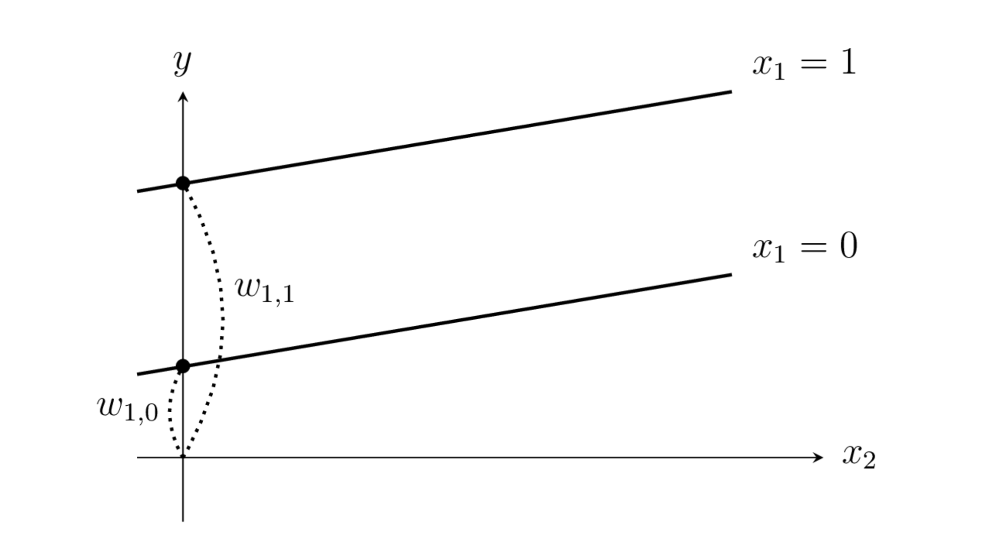
전체랭크모형의 경우 범주형 독립변수 chas가 \(d_{1,0}\), \(d_{1,1}\) 라는 두 개의 더미변수로 나뉘어진다.
chas = 0 인 경우, \(d_{1,0}=1\), \(d_{1,1}=0\)
chas = 1 인 경우, \(d_{1,0}=0\), \(d_{1,1}=1\)
예측식은 다음과 같아진다.
따라서 chas = 0 인 경우
chas = 1 인 경우
가 되어 x의 값에 따라 y절편이 달라지는 1차 모형이 된다.
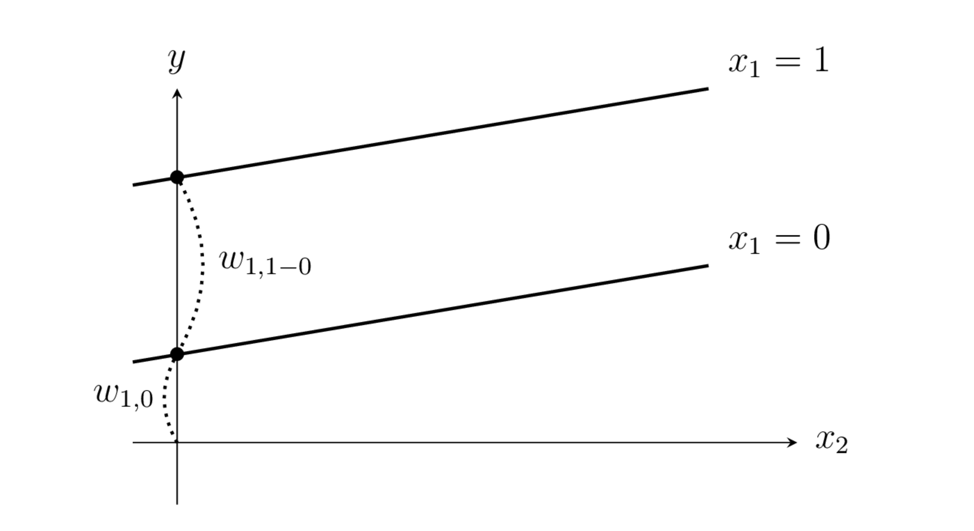
전체랭크모형의 경우 범주형 독립변수 chas가 \(d_{1,0}\), \(d_{1,1-0}\) 라는 두 개의 더미변수로 나뉘어진다.
chas = 0 인 경우, \(d_{1,0}=1\), \(d_{1,1-0}=0\)
chas = 1 인 경우, \(d_{1,0}=1\), \(d_{1,1-0}=1\)
예측식은 아까와 동일하다.
chas = 0 인 경우
chas = 1 인 경우
으로 chas = 0 인 경우 y 절편이 \( w_{1,0}\), chas = 0 인 경우 y 절편이 \(w_{1,0} + w_{1,1-0}\) 인 1차 식이 된다.
선형회귀 분석결과는 다음과 같다.
result5 = model5.fit()
print(result5.summary())
                            OLS Regression Results
==============================================================================
Dep. Variable:                   medv   R-squared:                       0.496
Model:                            OLS   Adj. R-squared:                  0.494
Method:                 Least Squares   F-statistic:                     247.6
Date:                Thu, 13 Oct 2022   Prob (F-statistic):           1.36e-75
Time:                        00:37:29   Log-Likelihood:                -1666.8
No. Observations:                 506   AIC:                             3340.
Df Residuals:                     503   BIC:                             3352.
Df Model:                           2
Covariance Type:            nonrobust
==============================================================================
                 coef    std err          t      P>|t|      [0.025      0.975]
------------------------------------------------------------------------------
C(chas)[0]    22.2504      0.301     73.799      0.000      21.658      22.843
C(chas)[1]    26.3330      1.110     23.723      0.000      24.152      28.514
scale(rm)      6.2944      0.292     21.555      0.000       5.721       6.868
==============================================================================
Omnibus:                       92.470   Durbin-Watson:                   0.753
Prob(Omnibus):                  0.000   Jarque-Bera (JB):              572.587
Skew:                           0.619   Prob(JB):                    4.62e-125
Kurtosis:                       8.062   Cond. No.                         3.83
==============================================================================

Notes:
[1] Standard Errors assume that the covariance matrix of the errors is correctly specified.
result6 = model6.fit()
print(result6.summary())
                            OLS Regression Results
==============================================================================
Dep. Variable:                   medv   R-squared:                       0.496
Model:                            OLS   Adj. R-squared:                  0.494
Method:                 Least Squares   F-statistic:                     247.6
Date:                Thu, 13 Oct 2022   Prob (F-statistic):           1.36e-75
Time:                        00:37:29   Log-Likelihood:                -1666.8
No. Observations:                 506   AIC:                             3340.
Df Residuals:                     503   BIC:                             3352.
Df Model:                           2
Covariance Type:            nonrobust
================================================================================
                   coef    std err          t      P>|t|      [0.025      0.975]
--------------------------------------------------------------------------------
Intercept       22.2504      0.301     73.799      0.000      21.658      22.843
C(chas)[T.1]     4.0825      1.151      3.547      0.000       1.821       6.344
scale(rm)        6.2944      0.292     21.555      0.000       5.721       6.868
==============================================================================
Omnibus:                       92.470   Durbin-Watson:                   0.753
Prob(Omnibus):                  0.000   Jarque-Bera (JB):              572.587
Skew:                           0.619   Prob(JB):                    4.62e-125
Kurtosis:                       8.062   Cond. No.                         3.98
==============================================================================

Notes:
[1] Standard Errors assume that the covariance matrix of the errors is correctly specified.